What I've Learned About AI in the Past Two Months.

This blog post was originally written in Chinese and translated into English entirely using ChatGPT o1. 如果想讀中文版，請滑到底。

Forward

I probably don’t need to say much about it—AI is changing the world at an astonishing pace. Ever since I read Ray Kurzweil’s The Singularity Is Near in 2019, upon the recommendation of a senior from my physics department, I have been convinced that I will witness the birth of Artificial Superintelligence (ASI) in my lifetime. However, over the past five years, most of my time and interests have been focused on startups and HCI research, and my AI knowledge remained at the level of Deep Learning with Python from back in 2018 when I was in the military. As a result, although I’ve used AI extensively in my work and personal life for the past two years, I haven’t had a deep understanding of the fundamental principles behind these technologies.

To remedy this gap and to have a more accurate view of technological developments, I set myself a goal starting in early November—over almost two months—to dive into the developments of AI over the past decade, understand the key technical principles involved, and think about how far we might still be from AGI and ASI. Although this research is still ongoing, I feel it’s time to share some of the interim results from my learnings.

Strictly speaking, this article is my “learning notes” from these two months, so it doesn’t have a true conclusion. Instead, it’s written in a more explanatory style, focusing on what I find most important and what I feel confident enough to share. My intended readers are friends who have some background in Deep Learning and are currently learning AI, so I won’t over-explain certain technical terms. I hope this learning note can offer some insightful narratives and perspectives on the current development of AI.

This article is divided into three parts. The first part explains the technical principles behind Large Language Models (LLMs), including Transformers and the Attention mechanism. I recommend watching some animated introductions to Transformers (particularly 3Blue1Brown’s Deep Learning videos #5 to #7) before reading that section. The second part discusses trends in LLM development over the past few years and explains why there is such a thing as the “Scaling Law.” The third part explores what AGI is, the relationship between LLMs and AGI, and which pieces might still be missing for humanity to create AGI.

Before we begin, I must emphasize that I am by no means an AI expert. I’m just a startup founder who has a background in math and physics and a strong interest in AI development. I’ve only spent three months in total studying AI theory—one month in May 2018, during my military service, when I read Deep Learning with Python, and these most recent two months, when I’ve read a lot of papers and watched countless YouTube videos, plus had countless conversations with ChatGPT. Therefore, if you find any errors or inaccuracies in this article, please do not hesitate to let me know.

RNN, Transformer, and Attention

In 2017, a team at Google Brain published the paper “Attention is All You Need,” which kicked off the LLM era. The primary goal of this paper was to address the seq2seq problem in language modeling—given an input sequence, you have to output another sequence, such as in Translation, Summarization, or Question Answering. A key characteristic of such problems is that both the input and output sequences can vary in length.

In Deep Learning, the most classic and commonly used model architecture for seq2seq problems is the Encoder-Decoder architecture. This means you first encode the input sequence into some representation via an Encoder, then decode that representation into an output sequence using a Decoder. Different models implement the Encoder and Decoder in different ways. Prior to 2017, the mainstream approach was to use recurrent architectures such as RNNs (or their variants, LSTM and GRU).

When using recurrent architectures to implement Encoders and Decoders, you feed in the tokens of the input sequence one by one during training. Taking the simplest RNN as an example, at time step t, the Encoder receives the input token x_t and the hidden state h_{t-1} from the previous time step, then outputs the hidden state h_t at the current time step. Because the computation at each time step depends on the hidden state from the previous step, you cannot parallelize the encoding of the entire input sequence. This becomes time-consuming for long input sequences. Moreover, since the Encoder “compresses” a long input sequence into the hidden state of the final time step (which is fixed in size and limited in the amount of information it can hold), the Decoder, when decoding that hidden state, is likely to lose a lot of information. While LSTM and GRU employ gating mechanisms to handle longer sequences, they still cannot fundamentally solve the issues of information loss with long sequences and lengthy training times.

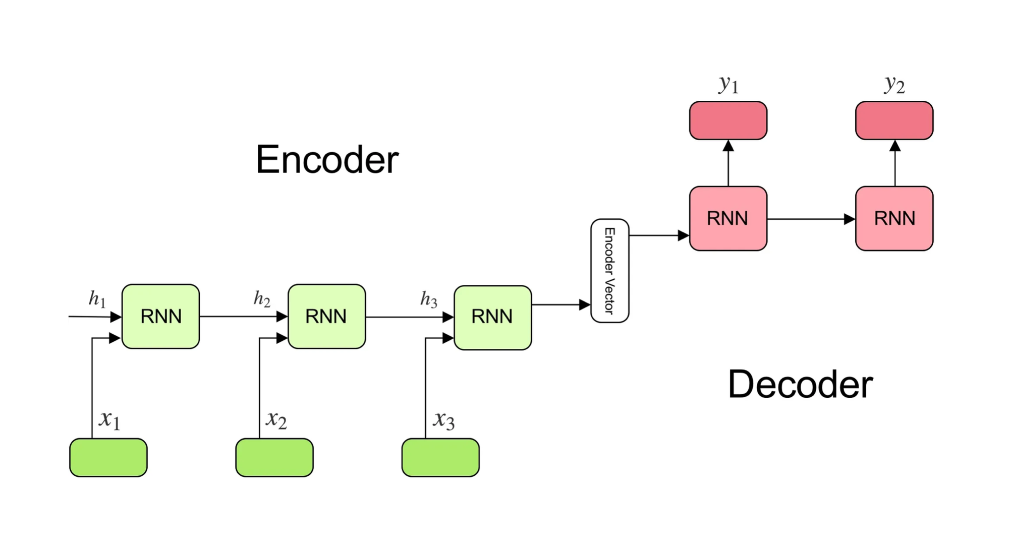
In 2014, Bahdanau et al. published “Neural Machine Translation by Jointly Learning to Align and Translate,” which first introduced the attention mechanism. With attention, the Decoder, when decoding, can consider not only the Encoder’s final hidden state but also the hidden states at every time step of the Encoder. It can dynamically decide, based on the current token, which hidden states to “pay more attention to.” This dramatically alleviates the problem of information loss over long sequences in recurrent-based Encoder-Decoder architectures and achieved better results in machine translation.

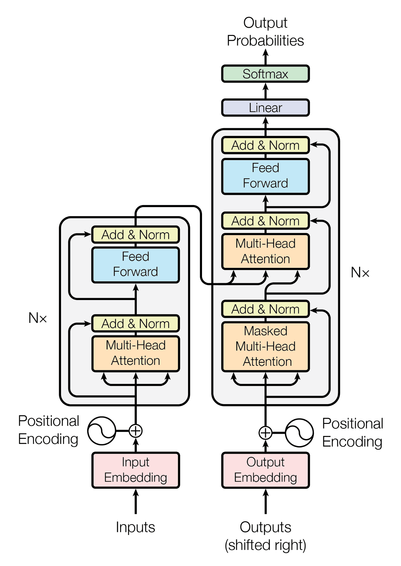
Returning to the “Attention Is All You Need” paper from 2017, its key finding was that we can discard RNNs entirely and implement both the Encoder and Decoder solely using attention, an architecture called the Transformer. In a Transformer, the Encoder first converts every token in the input sequence into an embedding vector in a high-dimensional space, then uses the self-attention mechanism to update (or “move”) these embedding vectors. Concretely, self-attention is implemented by training three matrices, W_q, W_k, and W_v. For the embedding vector of any token in the input sequence, you use these matrices to compute the corresponding query, key, and value vectors. Then, you take the query vector for this token, dot it with the key vectors of all tokens (and normalize) to obtain a distribution of attention weights, and use these weights to aggregate the value vectors of all tokens. This result becomes the update vector for the token’s embedding after the attention operation. This kind of embedding “update” is essentially what ResNet does with its residual connections.

For example, suppose each token is a single character. For the input sequence “I really want to eat”, you have five tokens. You can compute a 5×5 attention matrix by taking every token’s query vector and dotting it against every token’s key vector, which then indicates how much attention each token should pay to every other token. Finally, you use these attention weights to aggregate the value vectors and figure out how each token’s embedding should shift in vector space after self-attention.

Once the Encoder encodes the input sequence into embedding vectors processed by self-attention, the Decoder uses an auto-regressive approach to decode these vectors into an output sequence. Specifically, it continually treats the current time step’s output sequence as part of the input for the next time step, predicting the next token in a chain until a terminating token is predicted. When the Decoder does next-token prediction, it also applies self-attention to the current output sequence. However, there is an added mask mechanism so that each token can only “see” the tokens before it, preventing the Decoder from “cheating” by looking at the future tokens. This masking idea comes from Google DeepMind’s 2016 paper “Pixel Recurrent Neural Networks.”

After the Decoder sequence has been processed by self-attention, the Decoder performs cross-attention with the embedding vectors from the Encoder. That is, it computes the query vectors from the Decoder sequence while using the Encoder sequence to produce the key and value vectors. This allows the Decoder, when predicting the next token in the sequence, to simultaneously consider the content it has already decoded as well as the Encoder’s embeddings, and to dynamically allocate attention to the relevant parts of the Encoder’s output. For instance, if you’re translating Chinese into English, as the Decoder generates the English sequence, it uses cross-attention to decide which Chinese tokens in the Encoder it should pay the most attention to when predicting the next English token.

That covers the core mechanism of the Transformer. Other parts, such as Position Encoding and Feed Forward Networks, are more straightforward and are omitted here. In summary, the main advantage of Transformers is that they don’t rely on any recurrent architecture for the Encoder and Decoder, so the training can be parallelized. Meanwhile, the attention mechanism enables the model to effectively capture long-range token dependencies, solving the problems of information loss and poor performance in recurrent architectures for long sequences.

One additional point is that the Transformer paper introduced the concept of Multi-Head Attention. Whether in the Encoder or Decoder, the sequence undergoes attention across multiple sets of W_q, W_k, and W_v. Each set corresponds to one attention head. For a given token’s embedding, you sum up the update vectors provided by each attention head to get the final adjustment to that embedding. One way to think about this is that each attention head projects the embedding vector into a lower-dimensional subspace and “decides” token-to-token attention in a particular way. Different attention heads learn different patterns of attention, enabling the Transformer, as a whole, to learn more complex language patterns.

Since the publication of the Transformer paper, many modifications have been proposed to reduce computation cost and improve performance—such as Group Query Attention (retaining all query heads but reducing key and value heads), Multi Query Attention (keeping only one key and value head), or the Multi Latent Attention recently introduced by the Chinese company DeepSeek (which compresses all keys and values into a latent vector, then uses up-projection when needed). These are all tweaks to Multi-Head Attention that significantly reduce the memory needed for the KV cache.

Self-supervised Learning, Scaling Law, and Kolmogorov Compressor

The reason the advent of Transformers ushered in the LLM era is not only that they solved the issues of information loss and lengthy training times for recurrent-based models dealing with long sequences, but also because they addressed the problem of limited labeled data for training in the NLP field. Before 2017, Deep Learning had always been more advanced in Computer Vision (CV) than in NLP, largely thanks to ImageNet, which provided millions of labeled images. This allowed AI researchers to train models with huge amounts of labeled data. The success of AlexNet in 2012 (with about 60 million parameters) proved that the more labeled data you used to train bigger models, the better the performance—thus sparking the era of supervised learning. By contrast, NLP lacked large-scale, high-quality labeled datasets. Training recurrent-based models on unlabelled data was difficult to scale, so NLP lagged behind CV for a long time.

However, Transformers provided a scalable architecture for training language models on unlabelled data. Simply supply large volumes of real-world text, mask some of the words, and train the model to predict them. This is enough for the model to learn the internal structure of language representations. So, in 2018, just a year after Attention Is All You Need was published, OpenAI trained a Transformer Decoder on masses of unlabelled text for next-token prediction. They discovered that once the Decoder model was trained, you could fine-tune it with a small amount of labeled data for tasks like Sentiment Analysis, Question Answering, or Text Summarization, and it would perform very well. This was the earliest GPT (about 117 million parameters). Although the approach of pre-training and then fine-tuning was already widespread in CV, what made GPT unique was that its pre-training used unlabelled data—launching the era of self-supervised learning.

The next step was that everyone started making models bigger and bigger. Google used larger datasets to pre-train a Transformer Encoder, then fine-tuned it to release BERT, which performed much better than GPT. In response, OpenAI continued using the Decoder approach with bigger datasets and more parameters to create GPT-2 (about 1.5 billion parameters) and GPT-3 (about 175 billion parameters). They found that scaling the model’s size and dataset not only improved performance on many tasks without even needing to fine-tune—it also supported in-context learning by giving just a few examples in the prompt (few-shot). Google AI researcher François Chollet explained it as viewing an LLM as a continuous, “interpolative” program database, where all inputs and outputs are in an embedding space (e.g., a program called write_this_in_style_of_shakespeare could transform a poem into Shakespearean style). The larger the model, the more “programs” it contains, and a better prompt is more likely to locate and run the program best suited for the target task.

By this stage, the development of LLMs had entered a new phase. Beyond simply scaling model size and dataset, OpenAI began using instruction-tuning and RLHF (Reinforcement Learning from Human Feedback) on GPT-3.5 to teach the model to understand instructions and to give it a reward for outputs that align with human preferences—thus creating ChatGPT, which is highly useful to a general audience. GPT-4 can now handle multimodal inputs (e.g., images). All of these innovations—scaling model size and dataset in pre-training, supporting multimodality, fine-tuning, instruction-tuning, RLHF in post-training—have made LLMs increasingly “general,” prompting many to feel that AGI is coming closer.

Why does simply scaling a Transformer Decoder for next-token prediction produce such powerful LLMs? A talk given by Ilya Sutskever (OpenAI’s former Chief Scientist) at Berkeley offers insights. The key idea: “prediction,” “compression,” “learning,” “empirical induction,” and “pattern recognition” are essentially the same thing described in different ways. For instance, you can “learn” many “patterns” from real-world data, then “compress” that data into physics laws. Once you have physics laws, you can use them to “predict” various phenomena. A model that excels at prediction is a model that excels at finding the best compressor, which in turn means it’s good at learning and induction, compressing experiences into knowledge and forming an understanding of the world.

We can think of an LLM as a giant compressor. When you train the model, you’re effectively using stochastic gradient descent (SGD) to search for the ideal compression program. Interestingly, the theoretically best compressor is called the Kolmogorov compressor, which is Turing-incomputable. In practice, we can only approach it by scaling up the model size and training data via SGD, never actually reaching it. This is one intriguing explanation for why the scaling law works: as long as we have an endless supply of data, the model can keep getting better, though never perfect. Of course, in reality, we only have one internet, so it’s theoretically possible we’ll hit a wall if we use up all the internet data for pre-training.

If we understand LLMs as compressors, it becomes clearer why training on massive unlabelled data for next-token prediction followed by fine-tuning on small amounts of labeled data can be so effective. From the compressor’s perspective, compressing two datasets jointly always beats compressing them separately, because you can exploit shared structure between them to improve compression efficiency. If, by training on unlabelled data, the model has already learned most of the shared structure, then you’re effectively 99% of the way there; you naturally don’t need very much labeled data to achieve excellent results when fine-tuning for new language tasks.

Sequence Predictor, Search, and the Path of AGI

The emergence of LLMs makes many people feel that AGI is getting closer. But how close is it, really? What else do we need to build AGI? I think that before attempting to answer these questions, we need to define what we mean by “intelligence.” Personally, I agree with the definition given by Shane Legg (co-founder of Google DeepMind) in his doctoral dissertation, Machine Super Intelligence: Intelligence measures an agent’s ability to achieve goals in a wide range of environments. Put another way, you can’t just be good at Go; you have to be good at chess, be able to play video games, do math, write code, translate languages, diagnose diseases, conduct academic research, drive a car, etc. The broader your range of skills and the better you are at them, the more intelligence you have—the closer you are to “general intelligence.” Typically, when people talk about AGI, they’re referring to human-level AGI, meaning an AI that outperforms humans at nearly all tasks that humans excel at. Of course, some argue that an AI must surpass the global top 10 experts in each domain to qualify as AGI, while others argue that surpassing a 99th percentile benchmark in each domain is enough. Definitions vary by person.

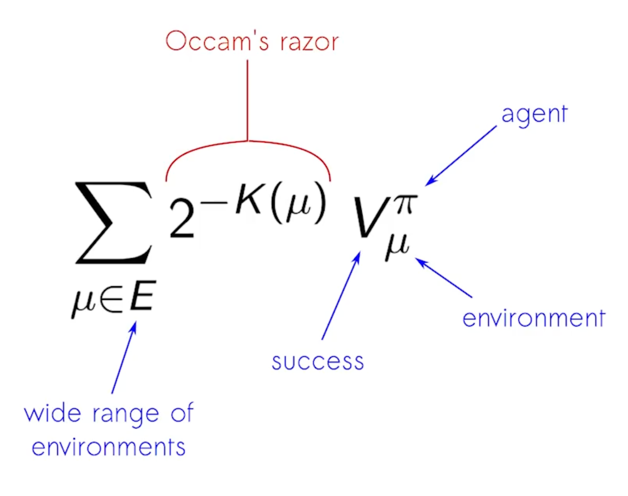
Returning to that definition—intelligence is about performing well across many environments and many goals. How do we measure intelligence? Shane Legg proposes evaluating an AI’s performance in every possible environment, then taking a weighted sum of these scores. The score in each environment is the expected discounted reward (per the Reinforcement Learning framework), and the weighting of scores across different environments follows Occam’s Razor. In other words, performance in simpler environments should carry more weight.

A simple example illustrates why Occam’s Razor is used to weight the scores. Imagine a simple IQ test question where the sequence is 01010, and you have to guess the next digit. The “correct” answer is 1. But theoretically, you could also come up with a sequence generator that produces 010100 as the first six digits. The reason we pick 1 is that we follow Occam’s Razor, which says if multiple generators can produce the prefix 01010, the simplest generator is the most likely to be correct. What do we mean by “simple?” Formally, if we find the shortest program that describes a sequence generator using a Universal Turing Machine, the program’s length is that generator’s Kolmogorov complexity (the “Kolmogorov compressor” we discussed earlier). The smaller the Kolmogorov complexity, the “simpler” the model.

Hence in Shane Legg’s formal definition of intelligence, he encodes the observations, actions, and rewards in each environment into an infinite sequence, and the length of the shortest program that generates that sequence is the environment’s Kolmogorov complexity. If that complexity is K, its score receives a weight of 2^(-K). In other words, performance in simpler environments has a larger weight. You can’t only be capable of handling complex tasks; you must also handle simple ones.

Of course, while elegant, such a formal definition poses practical limitations. First, Kolmogorov complexity is incomputable. Second, rather than building an AI that excels in every mathematically possible environment, we care more about whether it excels in the environments that matter to humans. So in practice, instead of using a Universal Turing Machine as a reference to weight performance across all environments, we might weight more heavily those environments with the greatest human, scientific, philosophical, or economic value.

With an operational definition of intelligence, we can revisit what we need for AGI. In the Reinforcement Learning framework, an AGI should be able to take any environment and quickly figure out the optimal action policy that maximizes the reward in that environment. So what properties would such an AGI have? Shane Legg’s doctoral advisor, Marcus Hutter, proposed an interesting theory in 2000 called AIXI, which I believe provides a useful thought experiment. Imagine you have unlimited compute resources at every moment—what could the most powerful AI agent do? The answer: from the limited historical data of that environment, it could identify the key regularities, then list all possible actions and, using those regularities, perform a brute-force search to compute the expected reward for each action, choosing the action with the highest expectation. Put differently, if we encode the environment’s observations, actions, and rewards into an infinite sequence, the most powerful AI agent needs two parts. First, it needs the theoretically most “sample-efficient” sequence predictor; second, it uses this predictor to do a brute-force search over all possible actions to find the optimal one.

What is the best theoretical sequence predictor? It’s called Solomonoff Induction. Recall the Occam’s Razor reasoning: if the sequence so far is 01010, the simplest explanation is that the next digit is 1. Solomonoff Induction doesn’t outright say the next digit is 1 but rather calculates the probability that it is 1. It does this by enumerating all possible programs that can generate the sequence 01010 and seeing which ones predict 1 and which predict 0. Programs with lower Kolmogorov complexity get higher probability weights. In short, AIXI is an AI agent that combines Solomonoff Induction with brute-force search.

Of course, in practice, we can’t build AIXI. Solomonoff Induction is Turing-incomputable, and we don’t have infinite compute to do brute-force search over all actions. Even so, AIXI is useful because it breaks AGI down into two core components: sequence prediction and search. AlphaGo and AlphaZero can’t exhaustively search every Go sequence but do use a UCT-based Monte Carlo Tree Search to beat Lee Sedol. ChatGPT, meanwhile, is essentially a massive next-token prediction engine. The key insight of the GPT series is that simply scaling model size and training data yields a better sequence predictor, leading to a more general AI chatbot that performs well across more tasks.

Recently, OpenAI introduced “o1,” and two weeks ago showcased “o3,” both of which incorporate reasoning. These models essentially combine a sequence predictor with search. Prior to o1, AI researchers noticed that adding a chain of thought in the prompt could endow the model with some reasoning capabilities—if you write out the reasoning steps you expect in the prompt, the LLM will try to follow that reasoning process. The better your chain of thought, the more likely you’ll get a correct answer. The unique feature of o1 is that, at test time, GPT first generates a tree of thought based on your prompt, then uses reinforcement fine-tuning to learn how to search for the chain of thought most likely to solve the problem, and finally feeds that chain of thought back into the LLM as a prompt. Referring to François Chollet’s interpretation of an LLM as a continuous, interpolative program database, this effectively does program synthesis from the programs stored in the LLM for new problems. This could improve o1’s performance on out-of-distribution problems, particularly something like ARC-AGI, which is designed to defeat memorization-based approaches.

It’s important to note that o1’s reinforcement fine-tuning differs from RLHF. RLHF uses an outcome reward model, which assigns a reward based on the quality of the final answer. Reinforcement fine-tuning also incorporates a process reward model, evaluating each step in the chain of thought during training. This helps the model more accurately estimate which chain of thought is more likely to produce a correct answer. You can find more details in the Awesome LLM Strawberry (OpenAI o1) repo, the paper “Scaling of Search and Learning: A Roadmap to Reproduce o1 from Reinforcement Learning Perspective,” or a video explanation by an Apple ML engineer.

Interestingly, OpenAI found that if you give the model exponentially more compute at test time to do the search, its reasoning ability improves linearly, allowing it to tackle more difficult problems. This is especially relevant for math, science, and engineering, where solutions are tough to find but easy to check for correctness. Put differently, scaling laws apply not just to pre-training but also to test-time compute. Hence, from o1 to o3, we see a major performance boost on many benchmarks. For instance, results improved on SWE-bench from 48.9% to 71.7%, Codeforce from 1891 to 2727, AIME from 83.3% to 96.7%, GPQA from 78.0% to 87.7%, ARC-AGI from 25% to 76%, and EpochAI Frontier Math from 2% to 25.2%.

I find these developments remarkable. Unlike pre-training, which takes a long time to produce a larger model, scaling test-time compute is still in its infancy. Only three months elapsed between the release of the o1 preview and the arrival of o3. For now, aside from GPU compute limits, there seems to be no major blocker to prevent AI giants from continuing to scale up test-time compute and build models with stronger reasoning capabilities. Of course, how well these models handle truly out-of-distribution problems—providing innovative solutions for tasks they’ve never seen—remains to be seen and requires continued observation.

What I find most inspiring about the o1 series is that its operation can be nicely mapped onto Daniel Kahneman’s theory in psychology. As François Chollet predicted in an interview with Dwarkesh Patel, the base model can be seen as a System 1 “intuitive response,” because it is trained with gradient descent as a parametric curve. It’s extremely fast and adept at pattern-matching but requires massive training data and can only do local generalization. On the other hand, the search at test time can be viewed as System 2 “thinking.” Because it is combinatorial, it requires less data but a great deal of computation to explore different combinations. When we combine the two, Deep Learning provides quick “intuition” that can vastly reduce the combinatorial explosion from brute-force searching. This neatly explains why spending more time “thinking” at test time lets the model solve more difficult problems.

Does scaling up LLM pre-training and test-time compute alone suffice to achieve human-level AGI? Yann LeCun, one of the three deep learning pioneers and Meta’s Chief AI Scientist, thinks not. He points out that a simple LLM lacks various capabilities we’d expect in a human-level AGI. For example, it has only a working memory within the context window—it lacks long-term episodic memory. It learns its multimodal capabilities from text-image datasets, but cannot, like humans, build a world model through interactions with the physical environment and use that model to plan future actions based on goals (like driving a car). Text is already a refined abstraction encoded in a limited symbol set; a human-level AGI should be able to derive abstractions from real-world interaction on its own.

While LLMs still have many limitations, self-supervised learning (which underpins them) will continue to be critical on the path to AGI. Take Yann’s JEPA (Joint-Embedding Predictive Architecture) project, aimed at next-frame prediction in videos. The core idea is not to predict every pixel of the next frame but to first encode the frames into abstract representations and then use self-supervised learning to predict on this abstraction layer, thus building a world model.

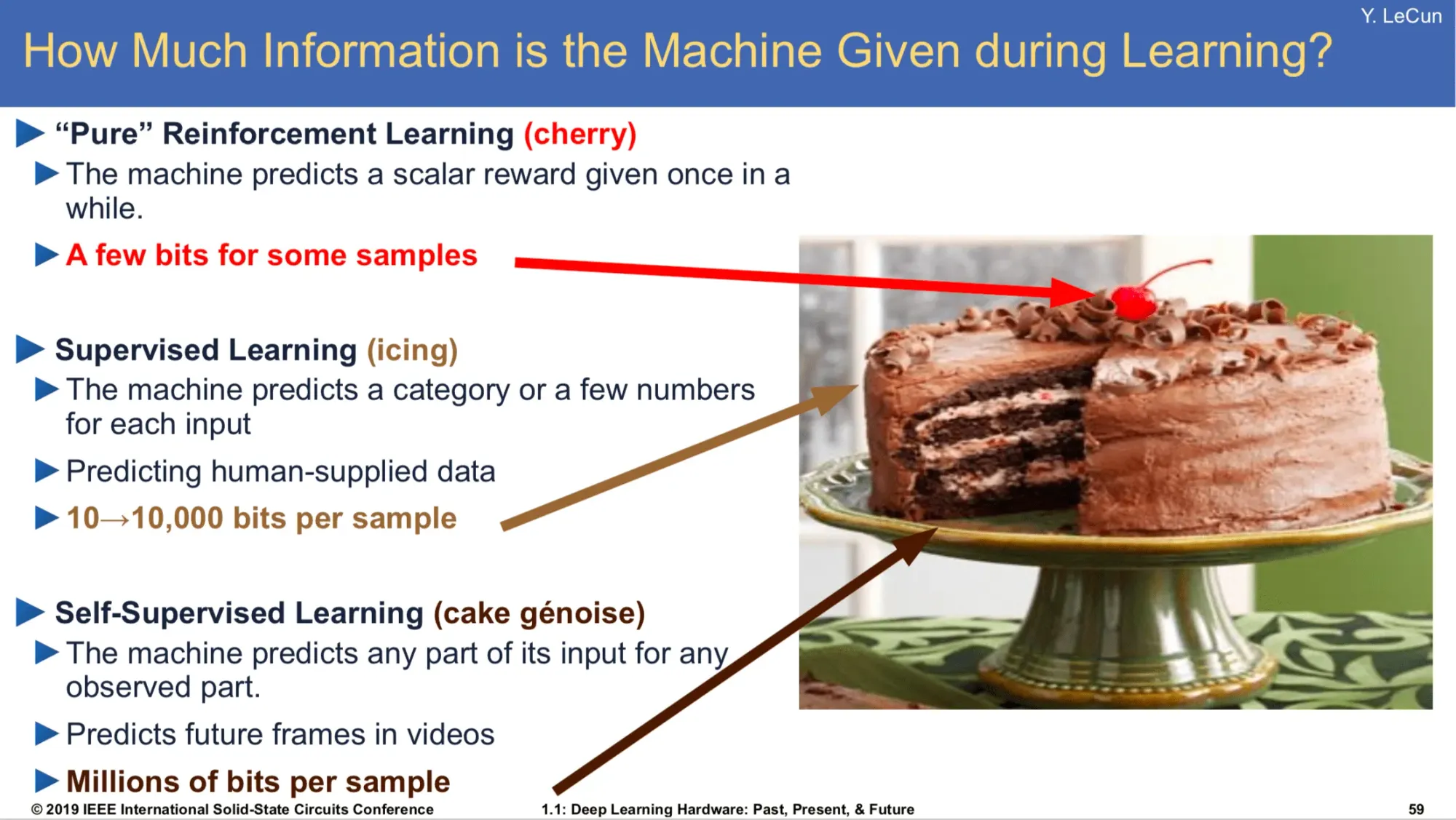
I don’t know whether JEPA will succeed, but to conclude this article, I’d like to share Yann LeCun’s analogy from his 2016 NeurIPS talk. This was before Attention Is All You Need was published, back when AlphaGo had just beaten Lee Sedol and Deep Reinforcement Learning was all the rage. LeCun said:

If intelligence is a cake, the bulk of the cake, the if you want, is unsupervised learning. The icing on the cake is supervised learning, and the cherry on the cake is reinforcement learning. And I must admit, this is slightly offensive to people who spend their days working on reinforcement learning. But I'll make it up, I promise. I'll make it up because there is a form of reinforcement learning that actually uses unsupervised learning as kind of a submodule, if you want.

In retrospect, this insight was remarkably forward-looking. The training approach of the o1 series models closely matches that cake analogy.

前言

相信不用我多說，AI 正在以驚人的速度改變世界。自從 2019 年在物理系學長的推薦下讀了 Ray Kurzweil 的《The Singularity Is Near》後，我便堅信自己會在有生之年見證超強人工智慧（ASI）的誕生。然而，過去五年我的時間和興趣主要投入在創業及人機互動的研究上，對 AI 的知識仍停留在 2018 年當兵時所讀的《Deep Learning with Python》。也因此，雖然這兩年我在工作和生活中大量使用 AI，卻對這些技術背後的實際運作原理了解有限。

為了彌補這樣的落差、也為了對科技的發展有更準確的認知，從 11 月初至今的近兩個月裡，我給自己設定了一個目標：深入研究過去十年 AI 的發展，了解其中的關鍵技術原理，並嘗試思考我們距離 AGI 和 ASI 究竟還有多遠。雖然這個研究目前仍在進行中，但我想也到了可以分享一些階段性學習成果的時候了。

這篇文章嚴格來說是我這兩個月的學習筆記，因此它沒有真正意義上的結論，而是採用更加解釋性的寫作方式去講解一些我覺得比較重要的、並且我比較有信心可以分享的相關知識。我的目標讀者是對 Deep Learning 有一定基礎、正在學習 AI 的朋友，因此有一些專有名詞不會多做解釋。我希望這篇學習筆記能為當前的 AI 發展提供一些啟發性的敘事與觀點。

這篇文章總共分成三個部分：第一部分會講大型語言模型（LLM）背後的技術原理，包含 Transformer 與 Attention 機制，我會建議先自己上網看一些跟 Transformer 有關的動畫介紹後再閱讀，這裡特別推薦 3Blue1Brown Deep Learning 系列的第五到七支影片。第二部分會講 LLM 在過去幾年的發展趨勢，並解釋為什麼會有 Scaling Law。第三部分會探討什麼是 AGI、LLM 與 AGI 的關係，以及人類在打造 AGI 可能還欠缺哪些東西。

在開始閱讀之前，我必須先強調：我絕對算不上什麼 AI 專家，只是一個擁有數學和物理的知識基礎、對 AI 發展非常感興趣的創業者。我真正花在學習 AI 理論上的時間只有 2018 年五月在當兵時讀的《Deep Learning with Python》，以及最近這兩個月看了大量 Paper 和 Youtube 影片，並與 ChatGPT 進行了無數次的對話。因此，如果你在本文中發現了任何錯誤或不精確之處，還請不吝指正。

RNN, Transformer, and Attention

2017 年，Google Brain 的團隊發佈了 Attention is All You Need 這篇 paper，開啟了 LLM 時代。這篇 paper 主要是在解決語言模型中 seq2seq 的問題，也就是給一串輸入的 sequence，要求輸出另一串 sequence，像是 Translation、Summary、Question Answering 都算是 seq2seq 的問題。這類問題的特點是 input sequence 和 output sequence 的長度都不是固定的。

Deep Learning 在解決 seq2seq 問題時最經典、常用的 model 架構是 Encoder-Decoder 架構，也就是先把 input sequence 透過 Encoder 編碼成特定的 representation，再用 Decoder 去將這個 representation 解碼成 output sequence。不同的 model 會用不同的方式實作 Encoder 和 Decoder，在 2017 年以前主流的做法是用 recurrent 的架構來實作，例如 RNN 或是它的變種 LSTM、GRU。

在用 recurrent 的架構實作 Encoder 和 Decoder 時，訓練階段會逐一讀入 input sequence 的每個 token。以最簡單的 RNN 為例，Encoder 在 time step t 會接收 input token x_t 和前一個 time step 輸出的 hidden state h_{t-1}，然後輸出該 time step 的 hidden state h_t。由於每個 time step 的運算都必須仰賴前一個 time step 的 hidden state，因此整段 input sequence 的編碼過程無法平行計算。這使得當 input sequence 很長時，訓練時間也會變得很長，並且由於 Encoder 將這個 long input sequence「壓縮」成了最後一個 time step 的 hidden state（長度固定、資訊量有限），使得 Decoder 在解碼這個 hidden state 時容易遺失許多資訊。雖然 LSTM 和 GRU 可以利用一些 gating 的機制處理更長的 sequence，但還是無法真正解決 long sequence 在經過 Encoder 後資訊遺失的問題以及訓練時間很長的問題。

在 2014 年，Bahdanau 等人發佈了 Neural Machine Translation by Jointly Learning to Align and Translate 這篇 paper，首次提出了 attention 的機制，也就是讓 Decoder 在解碼時不只看 Encoder 的最後一個 hidden state，而是可以同時參考 Encoder 在每個 time step 產生的 hidden state，並且在解碼過程根據當前的 token 動態地選擇要更加「注意」哪些 hidden state。這樣的作法大幅解決了 recurrent-based Encoder-Decoder 架構在處理 long sequence 時資訊遺失的問題，在機器翻譯問題上獲得了更好的表現。

回到 2017 年的 Attention is All You Need 這篇 paper，它最關鍵的發現在於我們可以把 RNN 全部丟掉，只用 attention 機制來實作 Encoder 和 Decoder 就足夠了，這個架構就叫 Transformer。在 Transformer 中，Encoder 會先把 input sequence 的每一個 token 轉成高維向量空間的 embedding vector，並利用 self-attention 機制去移動這些 embedding vectors。在這裡，self-attention 機制的具體實作方式是訓練三個矩陣 W_q, W_k, W_v。對於 input sequence 中的任何一個 token 的 embedding vector，你都可以拿這三個矩陣去計算出對應的 query vector、key vector 和 value vector，然後拿它的 query vector 去和所有 token 的 key vector 內積後 normalize 算出一組注意力分配的權重，再用這組權重來加權所有 token 的 value vector，進而算出這個 token 的 embedding vector 在經過 attention 運算後需要位移的向量。這種移動 embedding vector 的做法基本上就是 ResNet 的 residual connection。

舉例來說，假設每個 token 都是一個字，「我好想吃飯」這個 input sequence 有五個 token，你可以利用每一個 token 的 query vector 和 key vector 去計算出一個 5x5 的注意力方陣，進而得知對於每一個 token 來說，它應該分配多少注意力在其他 token 上。最後你再用這些注意力權重去加權 value vector 就可以算出每一個 token 的 embedding vector 在經過 self-attention 後要如何移動到新的位置。

在 Encoder 將 input sequence 編碼成經過 self-attention 處理過的 embedding vectors 後，Decoder 會將這些 embedding vectors 用 auto-regressive 的方式解碼成 output sequence，也就是說它會不斷地把當前 time step 輸出的 output sequence 當作是 Decoder 在下一個 time step 時的輸入，並且用 next-token prediction 的方式不斷地讓這個 output sequence 變長直到解碼完成（預測到代表終止符的 token）。Decoder 在做 next-token prediction 時，一樣會先讓當前 output sequence 的 embedding vectors 通過 self-attention，只不過這裡的 self-attention 機制會多一層 mask，讓每一個 token 只能「注意」到位在它「之前」的 token，這麼做的用意是避免 Decoder 在預測未來的 token 時可以偷看答案。這個 masking 的想法源自於 Google DeepMind 在 2016 年發表的 Pixel Recurrent Neural Networks 這篇 paper。

在 Decoder 的 sequence 經過 self-attention 後，Decoder 會拿這個 sequence 跟 Encoder 編碼過的 embedding vectors 做 cross-attention，也就是用 Decoder 的 sequence 計算 query vectors、Encoder 的 sequence 計算 key vectors 和 value vectors，使得 Decoder 在預測 sequence 的下一個 token 時可以同時考慮到當下已經解碼完成的內容和 Encoder 編碼過的內容，並動態地對 Encoder 的 embedding vectors 分配注意力。舉例來說，如果在實作的是中文翻英文的任務，Decoder 會在英文的 sequence 生成的過程中，透過 cross attention 去決定要預測下一個英文 token 時需要對 Encoder 的哪些中文 token 給予更高的注意力。

以上就是 Transformer 最核心的運作機制，其他像是 Position Encoding、Feed Forward Network 的部分因為比較直觀，這邊就省略介紹。總而言之，Transformer 的重點在於它不需要用任何 recurrent 的架構實作 Encoder 和 Decoder，這使得它的訓練可以平行計算。同時，Attention 的機制使得 model 能有效地捕捉到距離很遠的 token 之間的關係，解決了 recurrent 的架構在 sequence 很長時資訊流失、表現不佳的問題。

值得補充的是，Transformer 的 paper 中提出的架構是 Multi-Head Attention，也就是不管在 Encoder 還是 Decoder 中，sequence 在經過 attention 時會同時面對好幾組不同的 W_q, W_k, W_v，每一組 W_q, W_k, W_v 代表著一個 attention head，而對於一個 token 的 embedding vector 來說，將每一個 attention head 所給出的位移向量加總起來才是這個 embedding vector 最終要位移的向量。我覺得可以把每一個 attention head 視作是將 embedding vector 投影到低維向量空間中用「某一種方式決定 token 之間的注意力」，不同的 attention head 會學習到不同方式的注意力，使得 Transformer 作為整體可以學到更複雜的語言模式。

在 Transformer 的 paper 發布之後這幾年，人們為了降低計算成本和提高性能對它做了許多改良，像是 Group Query Attention（保留所有 query head，但是減少 key & value head）、Multi Query Attention（只留下一個 key & value head），或是最近有名的中國公司 DeepSeek 推出的 Multi Latent Attention（將所有 key & value 壓縮成 latent vector，需要時再做 up-projection）都是原本的 Multi-Head Attention 的改良版本，可以大幅減少 KV cache 需要的記憶體

Self-supervised Learning, Scaling Law, and Kolmogorov Compressor

Transformer 的出現之所以會開啟 LLM 時代，除了它解決 recurrent-based model 在處理 long sequence 時資訊遺失的問題以及訓練時間很長的問題以外，更重要的是它解決了過去 NLP 領域可以用來訓練的資料不足的問題。在 2017 年以前，Deep Learning 在 CV 領域上的表現之所以一直比 NLP 領域成熟，一個非常關鍵的原因是 ImageNet 的出現，讓 AI researcher 可以用上千萬張人工 labelled 好的圖片去訓練 model，2012 年 AlexNet 的成功（約 6000 萬參數）更是證明了只要用愈多的 labelled data 去訓練愈大的 model，表現就會愈好，也因此開啟了 Supervised Learning 的時代；相較之下，NLP 領域一直缺乏高品質且大規模的 labelled data，如果用 unlabelled data 去訓練 recurrent-based model 又難以 scale，所以發展長期落後 CV 領域。

然而，Transformer 的出現等於是提供了一種可以 scale 的、基於 unlabelled data 去訓練的語言模型架構，你只要給拿愈多真實世界中的文本，把其中一些文字 mask 掉後去訓練 model 對這些文字的預測能力，就足以讓 model 學會非常多語言內在結構的 representation。所以在 Attention is All You Need 的 paper 發布隔年，OpenAI 就拿一堆 unlabelled 的文本去訓練 Transformer 的 Decoder 做 next-token prediction，並發現用這種方式把 Decoder model 訓練好後，只要再用少量的 labelled data 去針對某些任務（例：Sentiment Analysis、Question Answering、Text Summarization 等） fine-tune 這個 model，model 在這些任務的表現就可以非常好，這就是最早的 GPT（約 1.17 億參數）。雖然這種先 pre-train 再 fine-tune 的做法在 CV 已經行之有年，但 GPT 最大的差別是在於它是用 unlabelled data 來完成 pre-training 的，開啟了 Self-supervised learning 的時代。

所以接下來發生的事情就是大家開始一直把模型愈做愈大：Google 拿了更大的 dataset 去 pre-train Transformer Encoder 後再 fine-tune 後推出 BERT，表現比 GPT 好很多；為了打敗 BERT，OpenAI 繼續用 Decoder 拿更大的 dataset 和更多的參數去訓練 GPT-2（約 15 億參數）、GPT-3（約 1750 億參數），並發現 model 的資料和參數愈大，對許多任務連 fine-tune 都不用了，你只要在 prompt 給幾個例子（few-shot）就可以達到 in-context learning。Google 的 AI Researcher François Chollet 解釋這件事情的方式，就是把 LLM 想像成一個連續的、可插值的（interpolative）的 program database，這些 program 的輸入和輸出都在 embedding space 裏頭（例如可能有一個 program 叫 write_this_in_style_of_shakespeare，它可以把一首詩轉換成莎士比亞的風格），愈大的 model 會有愈多的 program，而愈好的 prompt 愈能從這個 database 中找到並執行那些最有助於解決目標任務的 program。

到了這裡，LLM 的發展已經進入了另一個新階段：除了不斷去 scale model size 和 dataset 以外，OpenAI 也開始在 GPT-3.5 上使用 instruction-tuning 和 RLHF (Reinforcement Learning from Human Feedback) 的訓練方式去讓 model 聽得懂人類的 instruction，並在給出符合人類期望和偏好的 output 時獲得 reward，進而開發出對普羅大眾真正有用的 ChatGPT。而到了 GPT-4 時，model 已經可以支援 multi-modal 的輸入（像是圖片）。不管是在 pre-training 階段去 scale model size 和 dataset、支援 multi-modal，還是在 post-training 階段去做 fine-tuning、instruction-tuning、RLHF，都使得 LLM 變得愈來愈「通用」，這也讓許多人感覺 AGI 好像離我們愈來愈近了。

為什麼單純去 scale Transformer Decoder 做 next-token prediction 就能打造出如此強大的 LLM 呢？我覺得 OpenAI 前首席科學家 Ilya Sutskever 之前在 Berkeley 給的一場演講對我有很大的啟發。這裡比較關鍵的想法是所謂的預測、壓縮、學習、經驗歸納、模式辨識，指的其實都是同一件事情，只是用不同方式來描述。舉例來說，你可以從自然界的數據中「學習」到許多的「模式」、進而將這些數據「壓縮」成物理定律。有了物理定律後，你就可以通過計算來「預測」許多事情。一個模型擅長預測，代表它擅長找到一個非常好的壓縮器，也代表它非常善於學習和歸納經驗，將經驗壓縮成知識、建立對世界的理解。

所以我們可以把 LLM 比喻為一個巨大的壓縮器，而當你在 train model 時，其實就是在用隨機梯度下降法（SGD）去搜尋那個最理想的壓縮器的 program。有趣的是，最理想的壓縮器在數學上叫 Kolmogorov compressor，它是 Turing 不可計算的，因此在實務上我們只能通過不斷 scale model size 和 training data 來取得更好的表現，透過 SGD 去嘗試「接近」Kolmogorov compressor，但無法真正達到它。這是對於 scaling law 為什麼有效的其中一種很有意思的解釋，只要我們有無止盡的 data，model 就能一直變得更好，但永遠無法達到完美。當然，在現實世界中我們只有一個 internet，所以 pre-training 如果把整個 internet data 都用完後確實還是可能撞到牆。

如果用壓縮器的角度去理解 LLM，就更能理解為什麼使用大量 unlabelled data 去訓練 next-token prediction 後，只要再用少量的 labelled data 去針對不同任務 fine-tune 就可以達到很好的成效。對於壓縮器來說，二份資料如果一起壓縮，成效一定會比分開壓縮好，因為一起壓縮的時候，你可以透過抽取二份資料的共享結構來提高壓縮效率。如果 model 在拿 unlabelled data 去訓練 next-token prediction 的能力時已經把大部分的共享結構都學到了，那麽可能就等同於走完 99% 的路了，你自然不需要太多的 labelled data 就能在新的語言任務上做到很好的 fine-tuning 效果。

Sequence Predictor, Search, and the Path of AGI

LLM 的出現讓人們感覺 AGI 離我們愈來愈近了。但具體有多近呢？我們要打造 AGI 還需要做什麼呢？我覺得在嘗試回答這些問題之前，首先要先定義什麼是 Intelligence。我個人認同的是 Google DeepMind 的 co-founder Shane Legg 在他的博士論文 Machine Super Intelligence 中給的定義，也就是 Intelligence 衡量的是一個 Agent 是否能在許多不同環境中有效地達成許多不同的目標。換句話說，你不能只有圍棋下得好，你也要會下西洋棋、會打電動、會算數學、會寫程式、會翻譯各國語言、會診斷疾病、會做學術研究、會開車，你的 Intelligence 才會高、你才能算是真正的 General Intelligence。而我們在說 AGI 時，我們多數時候其實在說的是 Human-level AGI，也就是這個 AI 要在絕大多數人類擅長達成的目標上都做得比人類還要好。當然，有些人認為 AI 必須要在每個領域超越該領域全球 Top 10 的人才能算是 AGI，也有些人認為 AI 只要能在每個領域達到全球 PR99 就算是 AGI，這裡的定義就因人而異。

回到前述的定義：Intelligence 代表著能在許多不同環境中有效地達成許多不同的目標的能力。那 Intelligence 要怎麼測量？Shane Legg 的作法是讓一個 AI 在每個可能的環境都有一個分數，然後把這些分數加權。AI 在一個環境的得分基本上就是用 Reinforcement Learning 的框架去算它在這個環境未來得到的 discounted reward 的期望值，而 AI 在不同環境的得分的加權方式則是採用奧坎剃刀法則（Occam’s Razor），也就是 AI 在複雜度較低的環境中的得分應該獲得較高的權重。

我們可以用一個簡單的例子來理解為什麼要用奧坎剃刀法則來做分數的加權：想像一下你在做智力測驗，要預測 01010 後下一個數字是多少時，這題的「正確答案」會是 1。然而，為什麼是 1 呢？理論上我們也可以找到一個 sequence generator，生成的前六個數字是 010100 不是嗎？原因是人類在思考問題時會使用奧坎剃刀法則，也就是如果有許多種 sequence generator 都能生成前五個數字是 01010 的字串，我們會認為愈簡單的 sequence generator 就是愈可能正確的 sequence generator。至於什麼是「簡單」呢？從形式化的角度來看，如果我們能用 Universal Turing Machine 找到能描述這個 sequence generator 的 shortest program，那麽這個 program 的長度就是這個 sequence generator 的 Kolmogorov complexity（這個 shortest program 其實就是前面提到的 Kolmogorov compressor），而 Kolmogorov complexity 愈小的 model 就是愈「簡單」的 model。

也因此在 Shane Legg 對 Intelligence 的形式化定義中，他把每一個環境在每一個 time step 的 observation, action, reward 編碼成一個 infinite sequence，那麽能生成這個 infinite sequence 的 shortest program 的長度就是這個環境的 Kolmogorov complexity。如果一個環境的 Kolmogorov complexity 是 K，那在加權該環境的得分時就會乘上一個 2^(-K) 的權重，意味著 AI 在愈簡單的環境中的表現對於它的 Intelligence 是更重要的，你不能只會做複雜的事情、不會做簡單的事情。

當然，這種形式化的定義雖然漂亮，但卻存在實務上的缺點。首先，Kolmogorov complexity 是不可計算的；再者，比起打造一個能在所有可能的數學環境中表現良好的 AGI，我們人類更關注這個 AGI 在所有「人類在乎的環境」中是否表現良好。所以比起用 Universal Turing Machine 作為 reference machine 來加權 AI 在不同環境的得分，實務上我們可能會為那些在人類科學、哲學和經濟上有更高價值的環境賦予更高的得分權重。

有了對 Intelligence 的定義後，我們就能回頭看一下打造 AGI 需要做哪些事情了。從 Reinforcement Learning 的框架來看，AGI 就是你給它任何一個環境，它都能快速地找到最好的 action policy 來最大化那個環境給的 reward。這樣的 AGI 會具備什麼樣的性質呢？Shane Legg 的博士指導教授 Marcus Hutter 在 2000 年時提出了一個叫 AIXI 的理論，我認為它給出了一個很有用的思想實驗，那就是想像一下如果你每時每刻都享有無限的計算資源，你能打造的最強大的 AI Agent 能做到什麼事情？答案是它能從環境中的有限歷史數據中識別出關於這個環境的重要規律，接著把當下所有可採取的 action 通通列出來，然後根據它所發現的規律去用 brute-force search 的方式計算每一個 action 在未來所帶來的 reward 的期望值，並選擇期望值最高的 action。換句話說，如果我們用前述的方式將環境的 observation, action, reward 編碼成 infinite sequence，那最強大的 AI Agent 必須包含二個部分，首先你要有理論上最 sample efficient 的 sequence predictor，接著你拿這個 sequence predictor 去對所有可能的 action 做 brute-force search，就可以找到理論上最完美的 action。

什麼是理論上最強的 sequence predictor 呢？答案是一個叫 Solomonoff Induction 的東西。我們前面有提到奧坎剃刀法則，也就是在預測 01010 後面的數字時，下一個數字應該要是 1，因爲愈簡單的解釋就是愈可能的解釋。Solomonoff Induction 就是一種基於奧坎剃刀法則的歸納法，它並不會直接說下一個數字是 1，而是會計算出下一個數字是 1 的機率有多大，而它計算機率的方式其實就是窮舉所有可能產生 01010 的 program，看哪些下一個數字是 1、哪些下一個數字是 0，然後 Kolmogorov complexity 愈低的 program 在做機率加權時會獲得愈高的權重。而 AIXI 以一言以蔽之，就是把 Solomonoff Induction 和 brute-force search 結合的一個 AI Agent。

當然，我們在實務上不可能打造出 AIXI，因為 Solomonoff Induction 是 Turing 不可計算的，並且我們沒有無限的計算資源去對所有可能的 action 做 brute-force search。即便如此，AIXI 有用的地方在於它把 AGI 拆解成 sequence prediction 和 search 這二個關鍵部分。以 AlphaGo 和 AlphaZero 為例，它們雖然沒辦法窮舉所有的圍棋棋路，但還是可以用像是 UCT-based 的 Monte-Carlo Tree Search 打敗李世乭。再以 ChatGPT 為例，這些 LLM 本質上就是巨大的、專門做 next-token prediction 的 sequence predictor，而整個 GPT 系列的 model 最關鍵的 insight 就是你只要 scale model size 和 training data 就可以獲得更好的 sequence predictor，進而打造出更佳通用、能在更多不同任務表現良好的 AI Chatbot。

如果我們再看 OpenAI 最近推出的 o1、以及二週前剛展示的 o3，這些具備推理能力的 model 本質上也是一個 sequence predictor 加上 search 的模型。在 o1 推出以前，就有 AI researcher 發現我們可以透過在 prompt 中添加 chain of thought 來獲得一定程度的推理能力，也就是如果你把你期望的推理流程寫下來當作 prompt 餵給 LLM，LLM 給的回應就會嘗試去滿足這個推理流程，推理流程的 prompt 寫得愈好，你就愈有機會獲得正確答案。而 o1 獨特的地方就在於它會在 test time 時讓 GPT 先根據你的 prompt 去生成 tree of thought，並透過 Reinforcement fine-tuning 的訓練讓 model 學習如何在這個 tree 上 search 最有機會解決問題的 chain of thought，最後再把這個 chain of thought 當作 prompt 餵給 LLM。如果回頭看 François Chollet 將 LLM 視為連續、可插值的 program database 的比喻，這似乎就是在以 LLM 中的 program 為原料針對新穎問題做 program synthesis 的過程，而這樣的過程很可能有助於提高 o1 系列的 model 在面對 out-of-distribution 的問題時的解題能力，特別是 ARC-AGI 這種專門設計來對抗 memorization 的問題。

這裡需要特別注意，o1 的 Reinforcement fine-tuning 跟 RLHF 並不一樣。RLHF 用的是 outcome reward model，也就是針對 model 回答的答案好壞去給予 reward；Reinforcement fine-tuning 則結合了 process reward model 和 outcome reward model，也就是 training 時不只會去看 model 回答的答案是否正確，還會去對 model 使用的 chain of thought 的每一個 step 給予 reward，讓 model 能更加準確地評估哪一條 chain of thought 更有機會逼近問題的答案。更深入的細節可以參考 Awesome LLM Strawberry (OpenAI o1) 這個 repo 中的文獻、Scaling of Search and Learning: A Roadmap to Reproduce o1 from Reinforcement Learning Perspective 這篇 paper，或是 Apple 的 ML Engineer 拍的講解影片。

值得一提的是，OpenAI 發現如果讓 model 在 test time 時指數提高計算資源在做 search，model 的推理能力就會線性地變強、能解決更加困難的問題，特別是像數學、科學、工程這種 solution 很難找、但是 solution 是否正確很好判斷的問題。換句話說，scaling law 不只發生在 pre-training 階段，也發生在 test-time compute 階段。所以 o3 相較於 o1 在各大 benchmark 的表現都有顯著的提升，比方說 SWE-bench 從 48.9% 提高到 71.7%、Codeforce 從 1891 提高到 2727、AIME 從 83.3% 提高到 96.7%、GPQA 從 78.0% 提高到 87.7%、ARC-AGI 從 25% 提高到 76%、EpochAI Frontier Math 從 2% 提高到 25.2%。

我覺得這樣的發現是相當驚人的，因為不像 pre-training 要花非常多時間才能訓練出下一個更大的 model，test-time compute 的 scaling 還在非常早期，從 o1-preview 推出到 o3 推出只間隔了三個月。目前看起來除了 GPU 的算力上限以外，似乎沒有其他 major blocker 可以阻止 AI 大廠繼續透過 scale test-time compute 來打造推理能力更強的 model。當然，這些 model 在面對 out-of-distribution 的問題時的表現如何、是否能針對完全沒見過的問題類型提出新穎的解法，還是一件尚未定案、需要持續觀察的事。

不過 o1 系列 model 對我來說最具啟發性的部分，是它的運作方式可以在 Daniel Kahneman 的心理學理論上找到非常好的對照。正如同 François Chollet 在 Dwarkesh Patel 的訪談中所預測的，原本的 base model 可以視為系統一的直覺反應，因為是用 Deep Learning 的梯度下降法所 train 出來的 parametric curve，所以運算起來非常快、非常善於 pattern-matching，但缺點是訓練時需要用到非常多的 training data，並且只能在這個 curve 上做 local generalization；test-time compute 時的 search 則可以視為系統二的思考，這種 search 因為是組合式的，所以需要的 data 不多，但是因為要嘗試非常多種組合才能找到解法，在運算上非常沒效率。而當我們將二者結合起來時，就能有效地讓 Deep Learning 提供有用的「直覺」來大幅提高 search 的效率，避免出現 brute-force search 的 combinatorial explosion。這樣的對照似乎完美地解釋了為什麼當 model 在 test time 花愈多時間「思考」時，就能解決愈困難的問題。

光靠 LLM 在 pre-training 和 test-time compute 的 scaling law，我們就能打造出 Human-level AGI 了嗎？Deep Learning 三巨頭之一、Meta 的首席 AI 科學家 Yann LeCun 認為不行。他指出單純的 LLM 不具備許多 Human-level AGI 應該要有的能力，像是它只有在每一個 context window 中的工作記憶（working memory），但沒辦法像人類一樣有長期的情節記憶（episodic memory）；它的 multi-modal 能力是從圖文數據中訓練出來的，但沒辦法像人類一樣能在跟物理世界互動的過程中建立 world model、並利用這個 world model 去根據任務的目標去規劃未來要做的 action（例：開車）。文字是一種已經被提煉完成、用有限的符號集編碼而成的 abstraction，但 Human-level AGI 應該要能自己從與物理環境的互動中去提煉出這些 abstraction。

雖然 LLM 仍存在著許多限制，但是 LLM 用到的 self-supervised learning 在打造 AGI 的道路上應該還是會扮演著至關重要的角色。以 Yann 在研究的 JEPA（Joint-Embedding Predictive Architecture）為例，他想要做到影片的 next frame prediction，其核心思路就是不去 predict 下一個 frame 的每一個 pixel，而是把這些 frame 先用一個 Encoder 編碼成 abstract representation 後，再用 self-supervised learning 的方式去 train model 在這個 abstraction layer 上做 prediction 的能力，進而建立 world model。

JEPA 會不會成功我不知道，不過在這篇文章的最後，我想分享 Yann LeCun 在 2016 年 NeurIPS 給的演講。早在 Attention is All You Need 發表的前一年，那個 AlphaGo 剛打敗李世乭、Deep Reinforcement Learning 最火熱的年代，Yann LeCun 就用了一個蛋糕的比喻揭示了未來十年整個 AI 領域的發展方向：「如果把 Intelligence 想像成一塊蛋糕，那麼蛋糕的大部分，也就是主要部分，是 unsupervised learning；在蛋糕上塗的糖霜是 supervised learning；而放在蛋糕頂端的那顆櫻桃就是 reinforcement learning。我必須承認，這對於那些每天都在研究 reinforcement learning 的人而言，或許有點冒犯。但我承諾會彌補這件事，因為事實上，的確存在某種 reinforcement learning 形式，它會把 unsupervised learning 作為一種 submodule 來使用。」如今回頭看，這樣的見解真的十分有遠見，o1 系列的 model 的訓練方式確實跟這個蛋糕的比喻如出一轍。